pacman::p_load(ggpubr, performance, reshape2, sp,
sf, spdep, sfdep, stplanr, tidyverse, tmap)Take Home Exercise 2
1. Overview
As city-wide urban infrastructures such as public bus, mass rapid transits, public utilities and roads become digital, data sets obtained could be used as a framework for tracking movement patterns through space and time.
1.1 The Task
This exercise aims to reveals the urban mobility patterns of public bus transit through geospatial data science and analysis (GDSA), and spatial interaction models. ars The original data was downloaded on 18th November 2023 from LTA DataMall under Section 2.6 - Passenger Volume by Origin Destination Bus Stops. It records the number of trips by weekdays and weekends from origin to destination bus stops. For the purpose of this exercise, we will be using the August data - origin_destination_bus_202308.csv for Weekday Morning Peak (6-9am).
2. Data preparation
2.1 Install R packages
The code chunk below uses pacman:: p_load() to load and install the following libraries:
ggpubr: Used to create and customizeggplot2-based publication ready plotsperformance: Used for computing measures to access model quality that are not directly provided by R’s ‘base’ or ‘stats’ packages.reshape2: Used to restructure and aggregate datasf: Used for geospatial data handlingsp: Used for spatial dataspdep: Used to create spatial weights matrix objectssfdep: Used to integrate with'sf'objects and the'tidyverse'stplanr: Used to create geographic ‘desire lines’ from origin-destination (OD) datatidyverse: A collection of R packages use in everyday data analyses. It is able to support data science, data wrangling, and analysistmap: Used for thematic mapping where spatial data distributions are visualized.
2.2 Import and Load Dataset
For the purpose of this exercise, we will be using three data sets.
origin_destination_bus_202308.csv: A csv file containing information about all the bus stops currently being serviced by bus, which includes bus stop identifier, and location coordinates.Bus Stop Location. A geospatial file retrieved from LTA DataMallMaster Plan 2019 Subzone Boundary: A polygon feature layer in ESRI shapefile format.
2.2.1 Importing Aspatial data
First, we will import the Passenger Volume by Origin Destination Bus Stops data set for August by using readr::read_csv() and store it in variable odbus. Also, we will be using glimpse() report to reveal the data type of each field.
Point to note: ORIGIN_PT_CODE and DESTINATION_PT_CODE are in <chr> format.
Show the code
odbus <- read_csv("data/aspatial/origin_destination_bus_202308.csv")
glimpse(odbus)
Rows: 5,709,512
Columns: 7
$ YEAR_MONTH <chr> "2023-08", "2023-08", "2023-08", "2023-08", "2023-…
$ DAY_TYPE <chr> "WEEKDAY", "WEEKENDS/HOLIDAY", "WEEKENDS/HOLIDAY",…
$ TIME_PER_HOUR <dbl> 16, 16, 14, 14, 17, 17, 17, 17, 7, 17, 14, 10, 10,…
$ PT_TYPE <chr> "BUS", "BUS", "BUS", "BUS", "BUS", "BUS", "BUS", "…
$ ORIGIN_PT_CODE <chr> "04168", "04168", "80119", "80119", "44069", "4406…
$ DESTINATION_PT_CODE <chr> "10051", "10051", "90079", "90079", "17229", "1722…
$ TOTAL_TRIPS <dbl> 7, 2, 3, 10, 5, 4, 3, 22, 3, 3, 7, 1, 3, 1, 3, 1, …2.2.2 Importing Geospatial data
Thereafter, we will import the Bus Stops Location and Master Plan 2019 Subzone Boundary.
2.2.2.1 Import Bus Stop data
We will be using sf::st_read() to import and sf::st_transform() to ensure that the projected coordinate system is in the right format before storing in variable busstop.
busstop <- st_read(dsn = "data/geospatial",layer = "BusStop") %>%
    st_transform(crs = 3414)
Reading layer `BusStop' from data source
`/Users/smu/Rworkshop/jiawenoh/ISSS624/Take-Home_Ex/Take-Home_Ex02/data/geospatial'
using driver `ESRI Shapefile'
Simple feature collection with 5161 features and 3 fields
Geometry type: POINT
Dimension: XY
Bounding box: xmin: 3970.122 ymin: 26482.1 xmax: 48284.56 ymax: 52983.82
Projected CRS: SVY21Also, we will be using glimpse() report to reveal the data type of each field.
glimpse(busstop)Rows: 5,161
Columns: 4
$ BUS_STOP_N <chr> "22069", "32071", "44331", "96081", "11561", "66191", "2338…
$ BUS_ROOF_N <chr> "B06", "B23", "B01", "B05", "B05", "B03", "B02A", "B02", "B…
$ LOC_DESC <chr> "OPP CEVA LOGISTICS", "AFT TRACK 13", "BLK 239", "GRACE IND…
$ geometry <POINT [m]> POINT (13576.31 32883.65), POINT (13228.59 44206.38),…2.2.2.2 Import MPSZ data
Similarily, we used sf::st_read() to import and sf::st_transform() to ensure that the projected coordinate system is in the right format before storing in variable mpsz.
mpsz <- st_read(dsn = "data/geospatial",
                   layer = "MPSZ-2019") %>%
  st_transform(crs = 3414)
Reading layer `MPSZ-2019' from data source
`/Users/smu/Rworkshop/jiawenoh/ISSS624/Take-Home_Ex/Take-Home_Ex02/data/geospatial'
using driver `ESRI Shapefile'
Simple feature collection with 332 features and 6 fields
Geometry type: MULTIPOLYGON
Dimension: XY
Bounding box: xmin: 103.6057 ymin: 1.158699 xmax: 104.0885 ymax: 1.470775
Geodetic CRS: WGS 84We will be using glimpse() report to reveal the data type of each field
glimpse(mpsz)Rows: 332
Columns: 7
$ SUBZONE_N <chr> "MARINA EAST", "INSTITUTION HILL", "ROBERTSON QUAY", "JURON…
$ SUBZONE_C <chr> "MESZ01", "RVSZ05", "SRSZ01", "WISZ01", "MUSZ02", "MPSZ05",…
$ PLN_AREA_N <chr> "MARINA EAST", "RIVER VALLEY", "SINGAPORE RIVER", "WESTERN …
$ PLN_AREA_C <chr> "ME", "RV", "SR", "WI", "MU", "MP", "WI", "WI", "SI", "SI",…
$ REGION_N <chr> "CENTRAL REGION", "CENTRAL REGION", "CENTRAL REGION", "WEST…
$ REGION_C <chr> "CR", "CR", "CR", "WR", "CR", "CR", "WR", "WR", "CR", "CR",…
$ geometry <MULTIPOLYGON [m]> MULTIPOLYGON (((33222.98 29..., MULTIPOLYGON (…2.3 Data Wrangling
Looking at section 2.2.1, we noticed a few problem:
ORIGIN_PT_CODE: is in<chr>formatDESTINATION_PT_CODE: is in<chr>format
We will be using dplyr::mutate() to convert the <chr> data type to <fct> and store it in a new variable odbus_new.
Show the code
odbus_new <- odbus %>%
 mutate(ORIGIN_PT_CODE = as.factor(ORIGIN_PT_CODE),
        DESTINATION_PT_CODE = as.factor(DESTINATION_PT_CODE))

glimpse(odbus_new)
Rows: 5,709,512
Columns: 7
$ YEAR_MONTH <chr> "2023-08", "2023-08", "2023-08", "2023-08", "2023-…
$ DAY_TYPE <chr> "WEEKDAY", "WEEKENDS/HOLIDAY", "WEEKENDS/HOLIDAY",…
$ TIME_PER_HOUR <dbl> 16, 16, 14, 14, 17, 17, 17, 17, 7, 17, 14, 10, 10,…
$ PT_TYPE <chr> "BUS", "BUS", "BUS", "BUS", "BUS", "BUS", "BUS", "…
$ ORIGIN_PT_CODE <fct> 04168, 04168, 80119, 80119, 44069, 44069, 20281, 2…
$ DESTINATION_PT_CODE <fct> 10051, 10051, 90079, 90079, 17229, 17229, 20141, 2…
$ TOTAL_TRIPS <dbl> 7, 2, 3, 10, 5, 4, 3, 22, 3, 3, 7, 1, 3, 1, 3, 1, …Additionally, we confirmed that there are no missing values in the odbus_new data set.
any(is.na(odbus_new))[1] FALSE2.3.1 Data Extraction
2.3.1.1 Analytical Hexagon
To get a better representative of the traffic analysis zone (TAZ), we will create an analytical hexagon grid. With reference from Urban Data Palette, we will used the code chunk below and execute in the following sequence:
st_make_grid(): create a regular grid of spatial polygons. To reflect the distance from centre of the hexagon to its edge (375m), we will revise the cell width and height to c(750,750) to reflect the full diameter.st_sf(): convert the honeycomb grid object to an sf object. We used[mpsz$geometry]to identify hexagon grid that intersects.rowid_to_column(): add rowid as a column. Values in this column are the row IDs of each grid cell.lengths(st_intersects()): assigns the number of bus stops for each cell to a new column named ‘bus_stops’ in hex_grid.st_intersects()checks for intersections between two spatial objects.as.factor(): to coverts the ‘grid_id’ column from<int>to<fct>tmap_options(check.and.fix = TRUE): forcing the polygons to be closedtm_shape()+tm_polygons(): plot the honeycomb grid cells as polygons
Show the code
#create regular grid
honeycomb = st_make_grid(mpsz,c(750,750),what = "polygons", square = FALSE)

#convert our honeycomb grid into an sf object and add rowid
hex_grid <- st_sf(honeycomb[mpsz$geometry]) %>%
  rowid_to_column('grid_id')

#add no. of bus stops into hex_grid data frame
hex_grid$bus_stops = lengths(st_intersects(hex_grid, busstop))

#convert grid_id from int to fct
hex_grid$grid_id <- as.factor(hex_grid$grid_id)

#plotting of Master Plan 2019 Subzone Boundary in analytical hexagon
tmap_options(check.and.fix = TRUE) #force close polygon
tm_shape(hex_grid) +
  tm_polygons() +
 tm_layout(main.title = "Analytical Hexagon Grid",
            main.title.position = "center",
            main.title.size = 1,
            legend.height = 0.35,
            legend.width = 0.35,
            legend.outside = FALSE,
            legend.position = c("right", "bottom"),
            frame = FALSE) +
tm_borders(alpha = 0.3)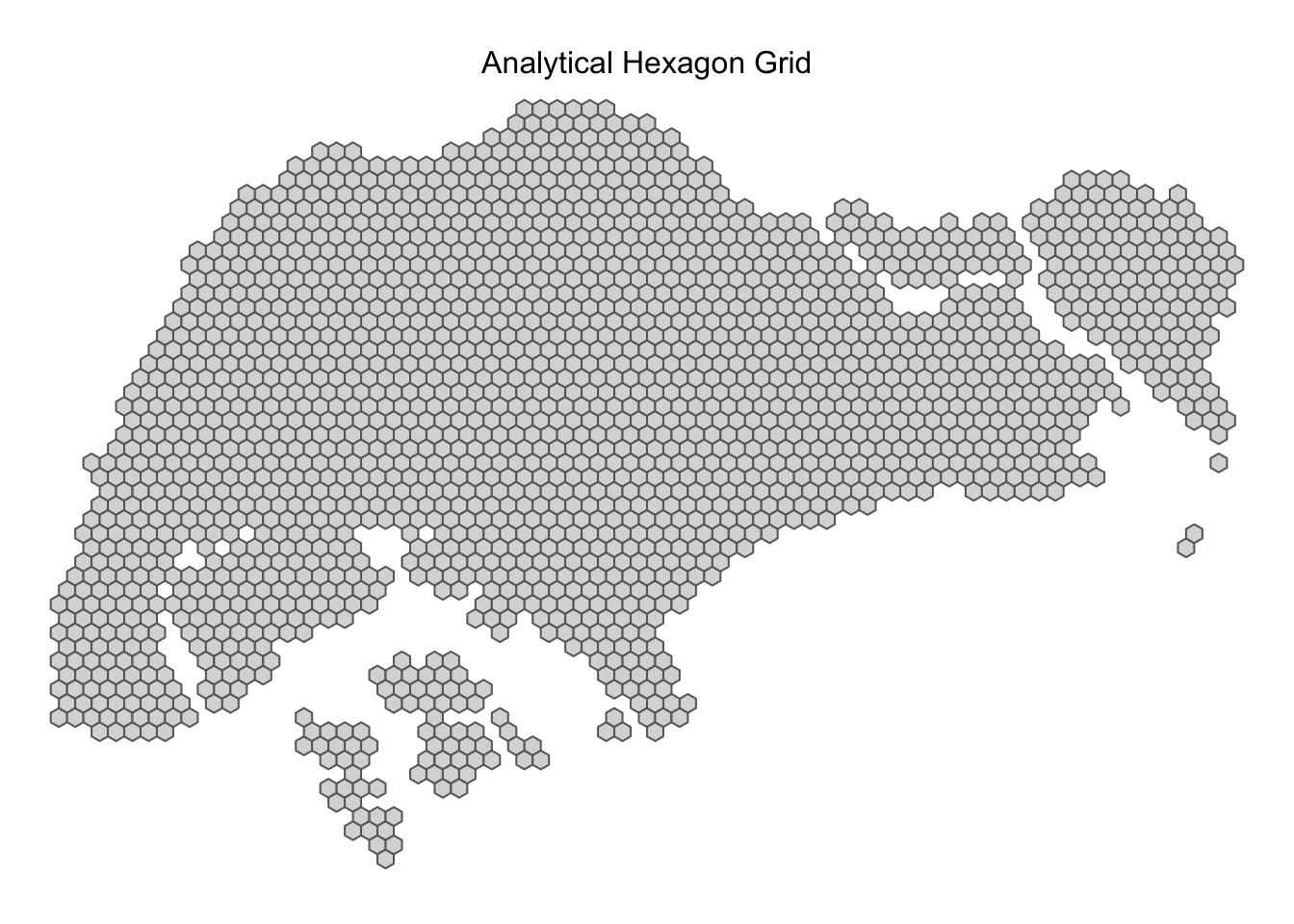
2.3.1.2 Commuting Flow
Through the previous exercise in Take Home Exercise 1, we were able to have a better understanding of the commuting flows. We noticed that the Peak hour period for Weekdays were generally higher as compared to Weekends, which we believe, could bring us more insights. As such, we will focus on our commuting flow at Weekday Morning Peak (6-9am).
The code is extracted in the following sequence:
filter()is used to extract subset of data for theDAY_TYPEandTIME_PER_HOURbetween()is used to express a range condition for theTIME_PER_HOURgroup_by()is used to grouped data. In our code, we will be grouping it based onORIGIN_PT_CODEandDESTINATION_PT_CODEsummarise()is used to sum the total number of tripsarrange(desc())is used to sort in descending orderungroup()is used to end a definition, often use withgroup_by()
Thereafter, we will save a copy of the output in rds format called wkd6_9.
Show the code
wkd6_9 <- odbus_new %>%
  filter(DAY_TYPE == "WEEKDAY",
         between(TIME_PER_HOUR, 6, 9)) %>%
  group_by(ORIGIN_PT_CODE, DESTINATION_PT_CODE) %>%
  summarise(TRIPS = sum(TOTAL_TRIPS)) %>%
  arrange(desc(TRIPS)) %>%
  ungroup()

#save a copy in RDS format
write_rds(wkd6_9, "data/rds/wkd6_9.rds")
As we are not executing the code chunk above, we will load wkd6_9 into the R environment.
wkd6_9 <- read_rds("data/rds/wkd6_9.rds")2.3.1.3 Visualing bus stops in hexagon grid
After importing the bus stop location in Section 2.2.2.1, we will create a visualization to observe the number of bus stops in each hexagon grid (grid_id). To get a better contrast, we incorporated RcolorBrewer into our code by adding a purple palette.
Show the code
#plot bus stop counts on hexagon layer
  tm_shape(hex_grid) +
  tm_fill(col = "bus_stops",palette = "Purples") +
  tm_layout(main.title = "Number of Bus Stops in Hexagon Grid",
            main.title.position = "center",
            main.title.size = 1,
            legend.height = 0.35,
            legend.width = 0.35,
            legend.outside = FALSE,
            legend.position = c("right", "bottom"),
            frame = FALSE) +
  tm_borders(alpha =0.3)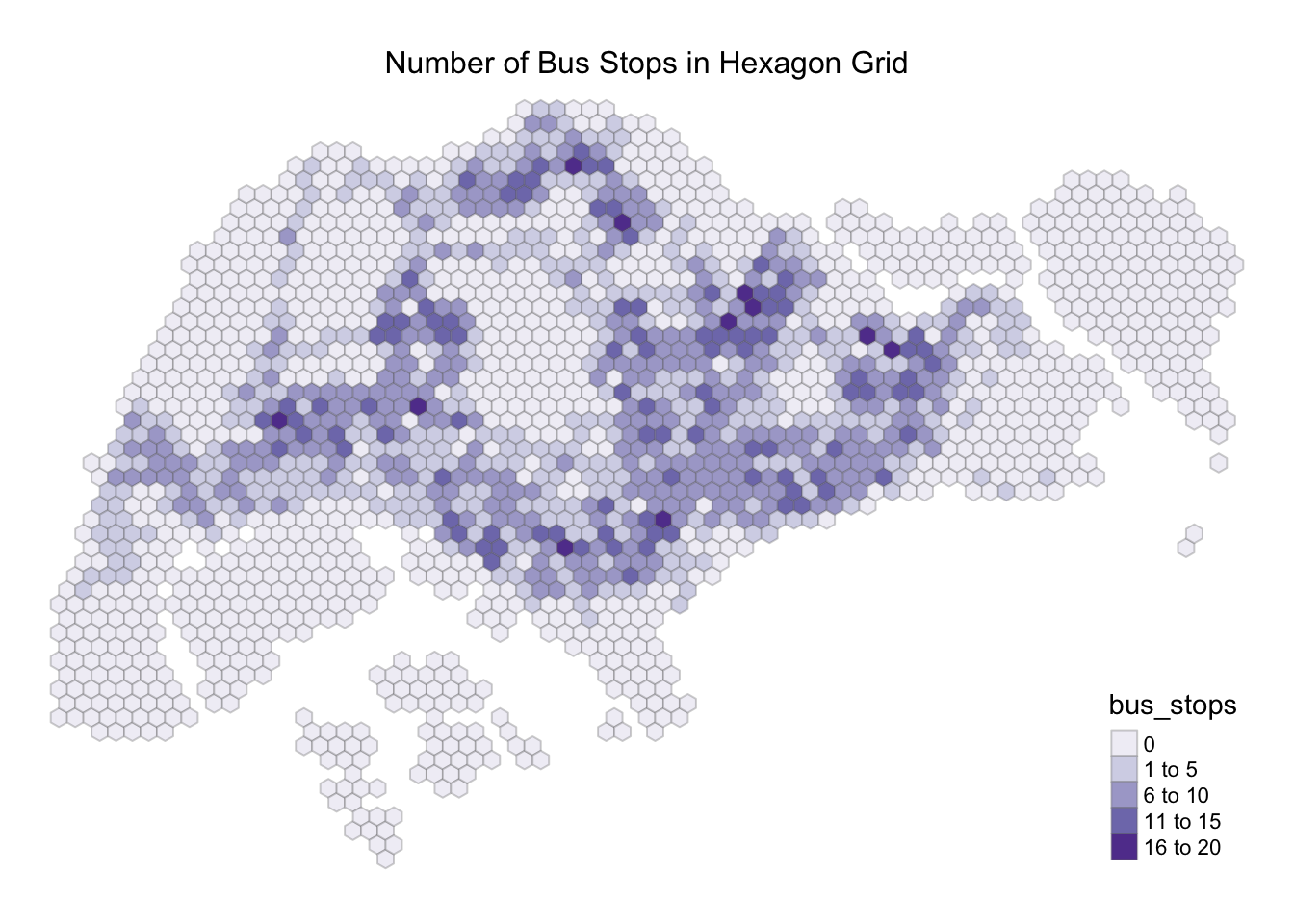
On average, we could see that most of the hexagon grids contain 6 to 10 bus stops with lesser dark colors hexagon grid as the data value increases. With the use of hexagon, we are able to identify the nearest neighbor by their common boundaries, infer that there might be some degree of influence as the colors does not differ significantly.
tm_shape() + Base Layer: Main plotting method. Used to specify a shape object.
-   Base Layer includes:

    -   `tm_polygons()`  - Create a polygon later (with borders)

    -   `tm_symbols()`  - Create a layer of symbols

    -    `tm_lines()`  - Create a layer of lines

    -    `tm_raster()`  - Create a raster layer

    -    `tm_text()`  - Create a layer of text labels

    -   `tm_basemap()`  - Create a layer of basemap tiles

- `tm_tiles()` - Create a layer of overlay tiles- Aesthetics derived layers, which includes:
-   `tm_fill()` :  - Create a polygon layer (without borders)

-   `tm_borders()` :  - Create a polygon borders

-   `tm_bubbles()` :  - Create a layer of bubbles

-   `tm_squares()` :  - Create a layer of squares

-   `tm_dots()` :  - Create a layer of dots

-   `tm_markers()` :  - Create a layer of markers

-   `tm_iso()` :  - Create a layer of iso/contour lines

-   `tm_rgb()` :  - Create a raster layer of an image
Facets
Attributes
Layout elements
Tmap_mode
For more information, click here.
2.4 Data Generation
2.4.1 Combining Busstop and mpsz
After extracting the commuting flow for Weekday Morning Peak, we will combine it into busstop sf data frame. To ensure distinct flows, we will use the unique() function into our code.
busstop_mpsz <- st_intersection(busstop, hex_grid) %>%
    select(BUS_STOP_N, grid_id) %>%
  st_drop_geometry()
Thereafter, we will perform the left_join() function twice. Firstly, we will join it based on ORIGIN_PT_CODE , where we will rename some of the columns and retain unique records. Then, we will join it based on DESTINATION_PT_CODE which we have renamed it as DESTIN_BS earlier.
After joining the data, we used drop_na() to removes any rows with missing values, and to group the data by origin and destination ID while computing the sum of trips for each origin-destination pair, saved under MORNING_PEAK. Lastly, a copy of the output - od_data was saved in RDS format.
Show the code
#left_join based on Origin_PT_Code
od_data <- left_join(wkd6_9 , busstop_mpsz,
            by = c("ORIGIN_PT_CODE" = "BUS_STOP_N")) %>%
  rename(ORIGIN_BS = ORIGIN_PT_CODE,
         ORIGIN_ID = grid_id,
         DESTIN_BS = DESTINATION_PT_CODE) %>%
  unique() %>%
  ungroup()

#left_join based on Destination_PT_code(rename as DESTIN_BS)
od_data <- left_join(od_data , busstop_mpsz,
            by = c("DESTIN_BS" = "BUS_STOP_N")) %>%
  unique() %>%
  ungroup()

# compute the morning peak trips between origin and destination grid
od_data <- od_data %>%
  rename(DESTIN_ID = grid_id) %>%
  drop_na() %>%
  group_by(ORIGIN_ID, DESTIN_ID) %>%
  summarise(MORNING_PEAK = sum(TRIPS)) %>%
  ungroup()

#save a copy in RDS format
write_rds(od_data, "data/rds/od_data.rds")
We will load od_data into the R environment.
od_data <- read_rds("data/rds/od_data.rds")2.4.2 Visualizing Spatial Interaction
With the joined data - od_data, we will prepare a desire line by using the stplanr package by removing the intra-zonal flows, creating the desire lines, and to visualize the desire lines.
2.4.2.1 Remove Intra-zonal flows
Intra-zonal flows refer to trips that take place within the same zone or area. In our context, it refers to the passenger commuting within the hexagon grid of 750m. As we will not be plotting the intra-zonal flows, the following code chunk below are used to only keep rows where the Origin_ID is not equal to the DESTIN_ID.
od_data1 <- od_data[od_data$ORIGIN_ID!=od_data$DESTIN_ID,]2.4.2.2 Create desire lines
Using the stplanr::od2line() function, we will create a line object where the flow refers to the data containing origin and destination information, zones refers to spatial data presenting the zone geometries, while zone_code refers to the specific column in our zones data that could identify the zone. In our case, it will be the grid_id. The output will be saved as flowLine.
flowLine <- od2line(flow = od_data1,
                    zones = hex_grid,
                    zone_code = "grid_id")
2.4.2.3 Visualizing desire lines
After creating the flowLine , we will visualize the resulting desire lines. Notably, quantiles provide a detailed picture of the how the MORNING_PEAK values are spread across. It allows us to identify if the flow is concentrated or evenly distributed across the network.
quantile(flowLine$MORNING_PEAK,
         probs = c(0.8, 0.9, 0.95, 0.99, 1))
80% 90% 95% 99% 100%
255.0 677.0 1479.0 6219.5 89347.0 From the results above, we will use tmap package to plot our visualization for the 80th percentile, 95% percentile, and 99% percentile. We began by plotting the background map tm_shape(hex_grid) + tm_polygons(), and filtering the flowLine to include flows based on the quantiles identified earlier. This allows us to focus on the most significant flow movements.
Afterwards, we used tm_shape() + tm_lines() to add flow lines into our visualization. In addition, we reduce the transparency of the lines to get a clear view of the flow. Low alpha results in transparency.
Show the code
tm_shape(hex_grid) +
  tm_polygons(col = 'grey95') +
flowLine %>%
    filter(MORNING_PEAK >= 255) %>%
tm_shape() +
  tm_lines(lwd = "MORNING_PEAK",  #set line width
           col = "purple",
           style = "quantile",
           scale = c(0.1, 1, 3, 5, 7, 10),
           n = 6,
           alpha = 0.8) +
    tm_layout(main.title = "Commuting flow of the top 20% ",
            main.title.position = "center",
            main.title.size = 1,
            legend.height = 0.35,
            legend.width = 0.35,
            legend.outside = FALSE,
            legend.position = c("right", "bottom"),
            frame = FALSE)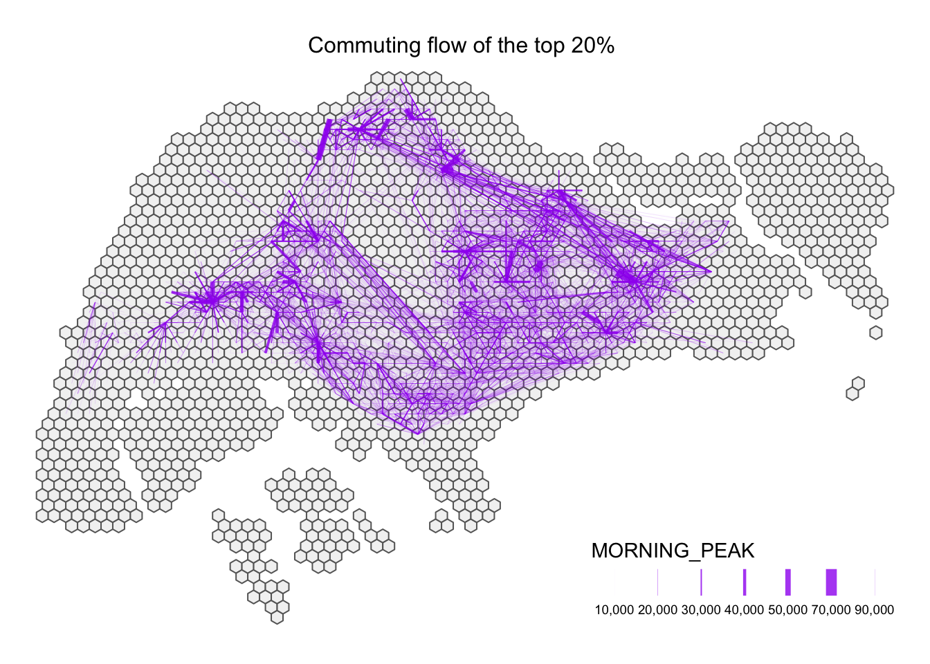
Show the code
tm_shape(hex_grid) +
  tm_polygons(col = 'grey95') +
flowLine %>%
    filter(MORNING_PEAK >= 1479) %>%
tm_shape() +
  tm_lines(lwd = "MORNING_PEAK",
           col = "purple",
           style = "quantile",
           scale = c(0.1, 1, 3, 5, 7, 10),
           n = 6,
           alpha = 0.8) +
    tm_layout(main.title = "Commuting flow of the top 5% ",
            main.title.position = "center",
            main.title.size = 1,
            legend.height = 0.35,
            legend.width = 0.35,
            legend.outside = FALSE,
            legend.position = c("right", "bottom"),
            frame = FALSE)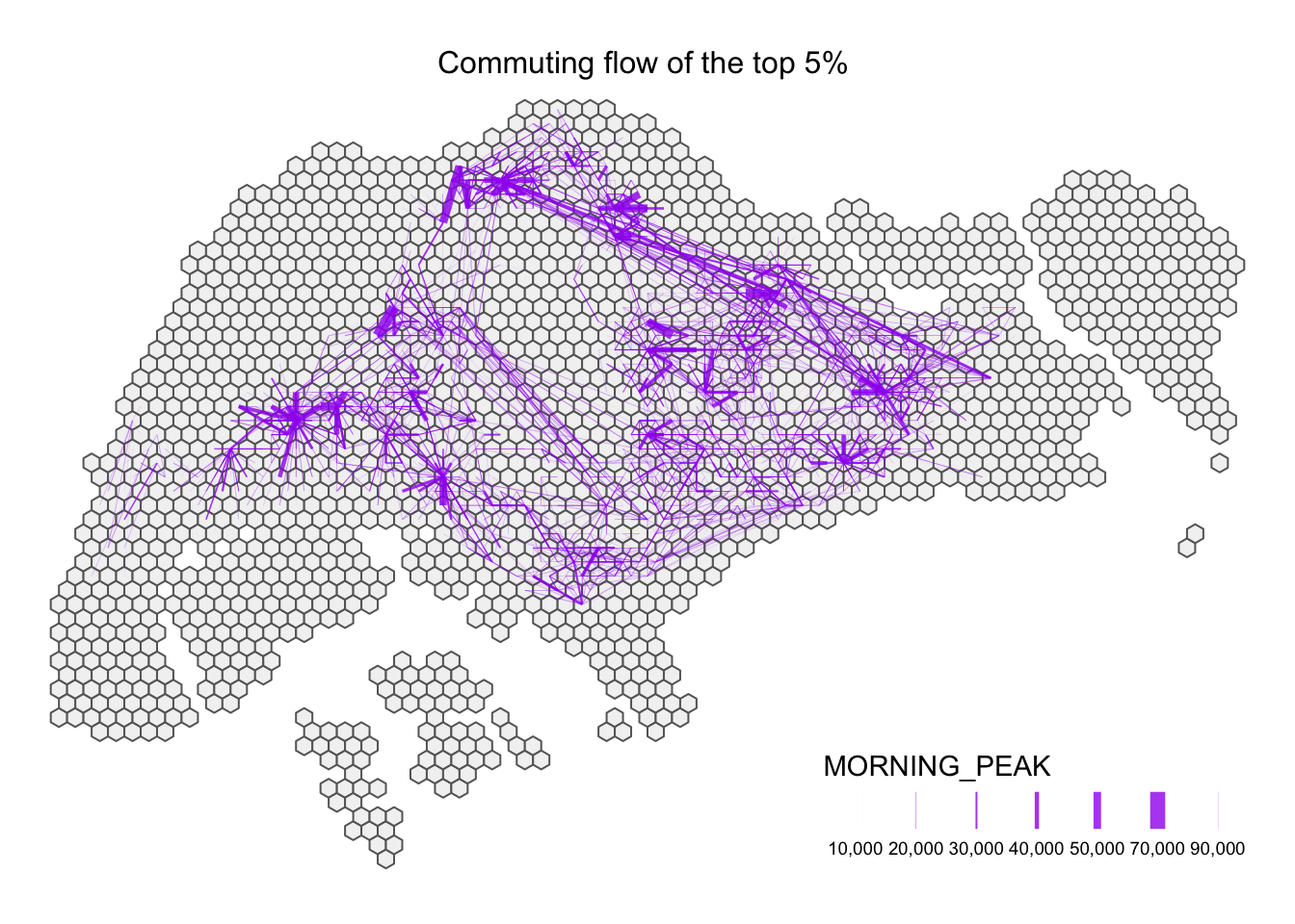
Show the code
tm_shape(hex_grid) +
  tm_polygons(col = 'grey95') +
flowLine %>%
    filter(MORNING_PEAK >= 6220) %>%
tm_shape() +
  tm_lines(lwd = "MORNING_PEAK",
           col = "purple",
           style = "quantile",
           scale = c(0.1, 1, 3, 5, 7, 10),
           n = 6,
           alpha = 0.8) +
    tm_layout(main.title = "Commuting flow of the top 1% ",
            main.title.position = "center",
            main.title.size = 1,
            legend.height = 0.35,
            legend.width = 0.35,
            legend.outside = FALSE,
            legend.position = c("right", "bottom"),
            frame = FALSE)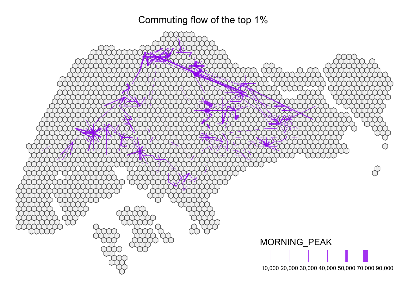
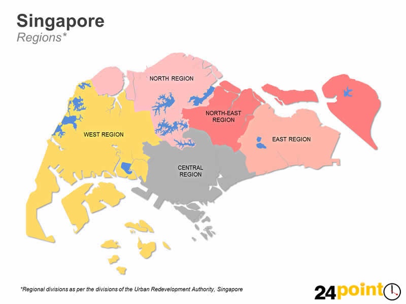
Based on the commuting flow of the 80th percentile, we could observe various clusters within the region, and commuters spend more travelling from origin to destination. From the thickness of the line, we could infer that the commuters travels the same route frequently - from the North region to the East region, and from the West region to the Central Region. It is interesting to note that commuters like myself do not travel from the West region to the East region frequently.
Looking at the 95th percentile , the flow movement decreased significantly. The commuting flow around the central region has dropped. Moreover, we are able to observe the flow from the North region to the East region, while we noticed that there are significant flow from the North region to the North-East region.
Narrowing it down to the top 1% (99% percentile), we are able identify that the longest commuting distance is from the North region to the North-East region. Also, commuters tend to travel within their region, travelling a short distance from origin to destination.
3. Data Integration
After looking at the commuting flows, we are interested to know why people traveled for a particular distance, and the purpose of their trip. Could it be for work? Could it be for school? As such, we will be importing eight collected data - Business, Entertainment, Food & Beverages, Financial Service, Leisure & Recreation, Retails, HDB and School as part of our mobility study.
3.1 Importing Collected Data
Similar to section 2.2, we used sf::st_read() to import and sf::st_transform() to ensure that the projected coordinate system is in the right format before storing it. With the exception of HDB and School data where we used readr::read_csv() to import and sf::st_as_sf() to converting an aspatial data into sf tibble data.frame.
Before we determine which exploratory variables are attractive or propulsive to a commuter, we plot a map based on the variables. We created a 3-layers plot by looking at :
Layer 1: Our base layer
(hex_grid). Hexagon grid with bus_stop density.Layer 2: Commuting flow movement. Identified based on purple lines.
Layer 3: Variables’ location. Identified based on blue dots.
By looking at the intersections between these layers, and our prior knowledge, we could better assemble the variables.
Show the code
business_sf <- st_read(dsn = "data/geospatial",
                      layer = "Business") %>%
      st_transform(crs = 3414)
Reading layer `Business' from data source
`/Users/smu/Rworkshop/jiawenoh/ISSS624/Take-Home_Ex/Take-Home_Ex02/data/geospatial'
using driver `ESRI Shapefile'
Simple feature collection with 6550 features and 3 fields
Geometry type: POINT
Dimension: XY
Bounding box: xmin: 3669.148 ymin: 25408.41 xmax: 47034.83 ymax: 50148.54
Projected CRS: SVY21 / Singapore TMShow the code
#plotting point symbol map with analytical hexagon grid
tmap_options(check.and.fix = TRUE)
tm_shape(hex_grid) +
  tm_fill(col = "bus_stops",palette = "Purples") +
tm_borders(alpha = 0.3) +
  flowLine %>%
    filter(MORNING_PEAK >= 1000) %>%
tm_shape() +
  tm_lines(lwd = "MORNING_PEAK",
           col = "purple",
           style = "quantile",
           scale = c(0.1, 1, 3, 5, 7, 10),
           n = 6,
           alpha = 0.8) +
    tm_layout(main.title = "Commuting flow of \n passengers with >1,000 trips",
            main.title.position = "center",
            main.title.size = 1,
            legend.height = 0.35,
            legend.width = 0.35,
            legend.outside = FALSE,
            legend.position = c("right", "bottom"),
            frame = FALSE) +
tm_shape(business_sf) +
  tm_dots(col = "lightblue") +
  tm_layout(main.title = "Business Spot",
            main.title.position = "center",
            main.title.size = 1,
            legend.height = 0.35,
            legend.width = 0.35,
            legend.outside = FALSE,
            legend.position = c("right", "bottom"),
frame = FALSE) 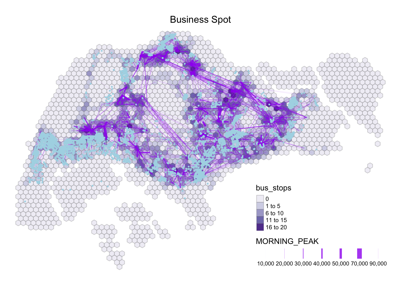
Show the code
entertn_sf <- st_read(dsn = "data/geospatial",
                      layer = "entertn") %>%
      st_transform(crs = 3414)
Reading layer `entertn' from data source
`/Users/smu/Rworkshop/jiawenoh/ISSS624/Take-Home_Ex/Take-Home_Ex02/data/geospatial'
using driver `ESRI Shapefile'
Simple feature collection with 114 features and 3 fields
Geometry type: POINT
Dimension: XY
Bounding box: xmin: 10809.34 ymin: 26528.63 xmax: 41600.62 ymax: 46375.77
Projected CRS: SVY21 / Singapore TMShow the code
#plotting point symbol map with analytical hexagon grid
tmap_options(check.and.fix = TRUE)
tm_shape(hex_grid) +
  tm_fill(col = "bus_stops",palette = "Purples") +
tm_borders(alpha = 0.3) +
    flowLine %>%
    filter(MORNING_PEAK >= 1000) %>%
tm_shape() +
  tm_lines(lwd = "MORNING_PEAK",
           col = "purple",
           style = "quantile",
           scale = c(0.1, 1, 3, 5, 7, 10),
           n = 6,
           alpha = 0.8) +
    tm_layout(main.title = "Commuting flow of \n passengers with >1,000 trips",
            main.title.position = "center",
            main.title.size = 1,
            legend.height = 0.35,
            legend.width = 0.35,
            legend.outside = FALSE,
            legend.position = c("right", "bottom"),
            frame = FALSE) +
tm_shape(entertn_sf) +
  tm_dots(col = "lightblue") +
  tm_layout(main.title = "Entertainment Spot",
            main.title.position = "center",
            main.title.size = 1,
            legend.height = 0.35,
            legend.width = 0.35,
            legend.outside = FALSE,
            legend.position = c("right", "bottom"),
frame = FALSE) 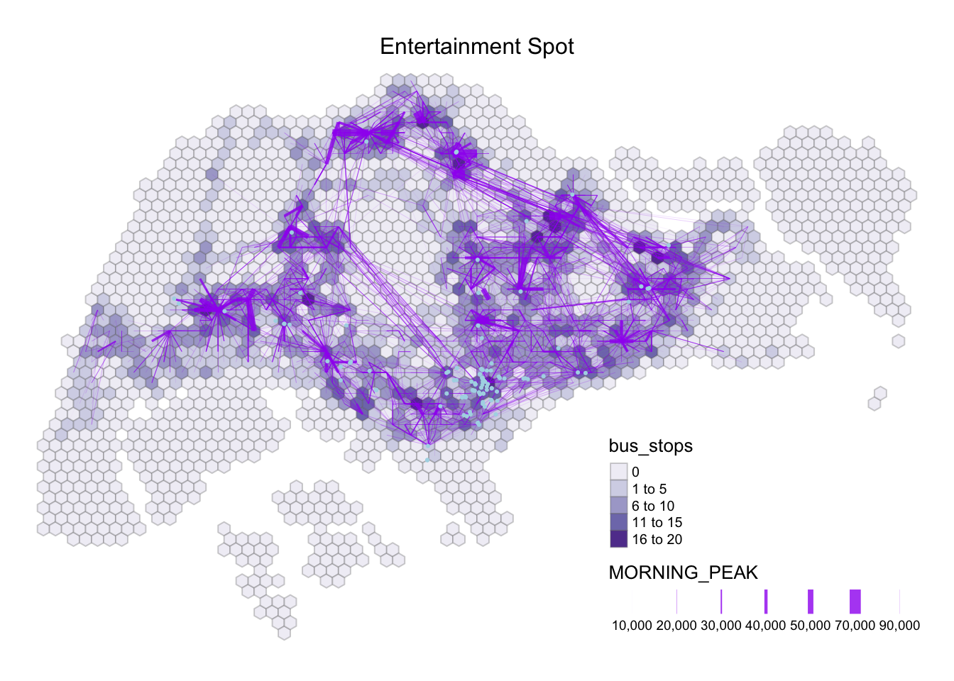
Show the code
fnb_sf <- st_read(dsn = "data/geospatial",
                      layer = "F&B") %>%
      st_transform(crs = 3414)
Reading layer `F&B' from data source
`/Users/smu/Rworkshop/jiawenoh/ISSS624/Take-Home_Ex/Take-Home_Ex02/data/geospatial'
using driver `ESRI Shapefile'
Simple feature collection with 1919 features and 3 fields
Geometry type: POINT
Dimension: XY
Bounding box: xmin: 6010.495 ymin: 25343.27 xmax: 45462.43 ymax: 48796.21
Projected CRS: SVY21 / Singapore TMShow the code
#plotting point symbol map with analytical hexagon grid
tmap_options(check.and.fix = TRUE)
tm_shape(hex_grid) +
  tm_fill(col = "bus_stops",palette = "Purples") +
tm_borders(alpha = 0.3) +
    flowLine %>%
    filter(MORNING_PEAK >= 1000) %>%
tm_shape() +
  tm_lines(lwd = "MORNING_PEAK",
           col = "purple",
           style = "quantile",
           scale = c(0.1, 1, 3, 5, 7, 10),
           n = 6,
           alpha = 0.8) +
    tm_layout(main.title = "Commuting flow of \n passengers with >1,000 trips",
            main.title.position = "center",
            main.title.size = 1,
            legend.height = 0.35,
            legend.width = 0.35,
            legend.outside = FALSE,
            legend.position = c("right", "bottom"),
            frame = FALSE) +
tm_shape(fnb_sf) +
  tm_dots(col = "lightblue") +
  tm_layout(main.title = "Food and Beverages Spot",
            main.title.position = "center",
            main.title.size = 1,
            legend.height = 0.35,
            legend.width = 0.35,
            legend.outside = FALSE,
            legend.position = c("right", "bottom"),
frame = FALSE) 
Show the code
finserv_sf <- st_read(dsn = "data/geospatial",
                      layer = "FinServ") %>%
      st_transform(crs = 3414)
Reading layer `FinServ' from data source
`/Users/smu/Rworkshop/jiawenoh/ISSS624/Take-Home_Ex/Take-Home_Ex02/data/geospatial'
using driver `ESRI Shapefile'
Simple feature collection with 3320 features and 3 fields
Geometry type: POINT
Dimension: XY
Bounding box: xmin: 4881.527 ymin: 25171.88 xmax: 46526.16 ymax: 49338.02
Projected CRS: SVY21 / Singapore TMShow the code
#plotting point symbol map with analytical hexagon grid
tmap_options(check.and.fix = TRUE)
tm_shape(hex_grid) +
  tm_fill(col = "bus_stops",palette = "Purples") +
tm_borders(alpha = 0.3) +
    flowLine %>%
    filter(MORNING_PEAK >= 1000) %>%
tm_shape() +
  tm_lines(lwd = "MORNING_PEAK",
           col = "purple",
           style = "quantile",
           scale = c(0.1, 1, 3, 5, 7, 10),
           n = 6,
           alpha = 0.8) +
    tm_layout(main.title = "Commuting flow of \n passengers with >1,000 trips",
            main.title.position = "center",
            main.title.size = 1,
            legend.height = 0.35,
            legend.width = 0.35,
            legend.outside = FALSE,
            legend.position = c("right", "bottom"),
            frame = FALSE) +
tm_shape(finserv_sf) +
  tm_dots(col = "lightblue") +
  tm_layout(main.title = "Financial Service Spot",
            main.title.position = "center",
            main.title.size = 1,
            legend.height = 0.35,
            legend.width = 0.35,
            legend.outside = FALSE,
            legend.position = c("right", "bottom"),
frame = FALSE) 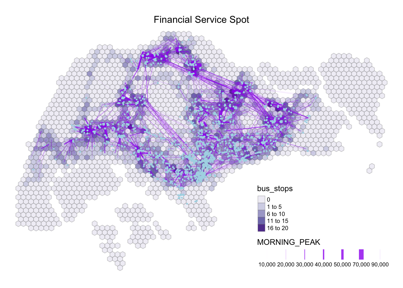
note that some residential area have commercial etc, would be a mixed development but we will include it in our analysis.
Show the code
#import hdb.csv and tidy data
hdb <- read_csv("data/aspatial/hdb.csv") %>%
  rename(latitude = "lat",
         longitude = "lng") %>%
  filter(residential == "Y")

#converting an aspatial data into sf tibble data.frame
hdb_sf <- st_as_sf(hdb,
                       coords = c("longitude", "latitude"),
                       crs=4326) %>%
  st_transform(crs = 3414)

#identify intersection between hdb and hex_grid to compute total_dwelling units
hdb_sf_sum <- st_intersection(hdb_sf, hex_grid) %>%
  group_by(grid_id) %>%
  summarise(
    HDB_SUM = sum(total_dwelling_units)
  ) %>%
  ungroup()

#plotting point symbol map with analytical hexagon grid
tmap_options(check.and.fix = TRUE)
tm_shape(hex_grid) +
  tm_fill(col = "bus_stops",palette = "Purples") +
tm_borders(alpha = 0.3) +
    flowLine %>%
    filter(MORNING_PEAK >= 1000) %>%
tm_shape() +
  tm_lines(lwd = "MORNING_PEAK",
           col = "purple",
           style = "quantile",
           scale = c(0.1, 1, 3, 5, 7, 10),
           n = 6,
           alpha = 0.8) +
    tm_layout(main.title = "Commuting flow of \n passengers with >1,000 trips",
            main.title.position = "center",
            main.title.size = 1,
            legend.height = 0.35,
            legend.width = 0.35,
            legend.outside = FALSE,
            legend.position = c("right", "bottom"),
            frame = FALSE) +
tm_shape(hdb_sf_sum) +
  tm_dots(col = "lightblue") +
  tm_layout(main.title = "HDB Spot",
            main.title.position = "center",
            main.title.size = 1,
            legend.height = 0.35,
            legend.width = 0.35,
            legend.outside = FALSE,
            legend.position = c("right", "bottom"),
frame = FALSE) 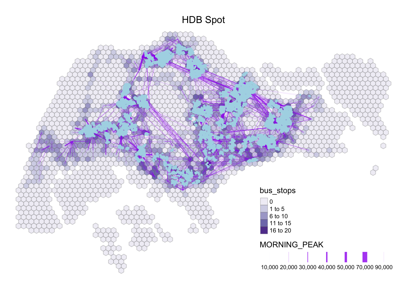
Show the code
lnr_sf <- st_read(dsn = "data/geospatial",
                      layer = "Liesure&Recreation") %>%
      st_transform(crs = 3414)
Reading layer `Liesure&Recreation' from data source
`/Users/smu/Rworkshop/jiawenoh/ISSS624/Take-Home_Ex/Take-Home_Ex02/data/geospatial'
using driver `ESRI Shapefile'
Simple feature collection with 1217 features and 30 fields
Geometry type: POINT
Dimension: XY
Bounding box: xmin: 6010.495 ymin: 25134.28 xmax: 48439.77 ymax: 50078.88
Projected CRS: SVY21 / Singapore TMShow the code
#plotting point symbol map with analytical hexagon grid
tmap_options(check.and.fix = TRUE)
tm_shape(hex_grid) +
  tm_fill(col = "bus_stops",palette = "Purples") +
tm_borders(alpha = 0.3) +
    flowLine %>%
    filter(MORNING_PEAK >= 1000) %>%
tm_shape() +
  tm_lines(lwd = "MORNING_PEAK",
           col = "purple",
           style = "quantile",
           scale = c(0.1, 1, 3, 5, 7, 10),
           n = 6,
           alpha = 0.8) +
    tm_layout(main.title = "Commuting flow of \n passengers with >1,000 trips",
            main.title.position = "center",
            main.title.size = 1,
            legend.height = 0.35,
            legend.width = 0.35,
            legend.outside = FALSE,
            legend.position = c("right", "bottom"),
            frame = FALSE) +
tm_shape(lnr_sf) +
  tm_dots(col = "lightblue") +
  tm_layout(main.title = "Leisure and Recreation Spot",
            main.title.position = "center",
            main.title.size = 1,
            legend.height = 0.35,
            legend.width = 0.35,
            legend.outside = FALSE,
            legend.position = c("right", "bottom"),
frame = FALSE) 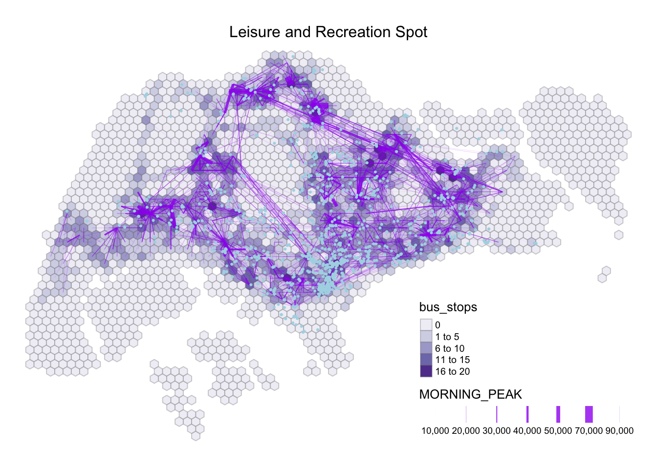
Show the code
retail_sf <- st_read(dsn = "data/geospatial",
                      layer = "Retails") %>%
      st_transform(crs = 3414)
Reading layer `Retails' from data source
`/Users/smu/Rworkshop/jiawenoh/ISSS624/Take-Home_Ex/Take-Home_Ex02/data/geospatial'
using driver `ESRI Shapefile'
Simple feature collection with 37635 features and 3 fields
Geometry type: POINT
Dimension: XY
Bounding box: xmin: 4737.982 ymin: 25171.88 xmax: 48265.04 ymax: 50135.28
Projected CRS: SVY21 / Singapore TMShow the code
#plotting point symbol map with analytical hexagon grid
tmap_options(check.and.fix = TRUE)
tm_shape(hex_grid) +
  tm_fill(col = "bus_stops",palette = "Purples") +
tm_borders(alpha = 0.3) +
    flowLine %>%
    filter(MORNING_PEAK >= 1000) %>%
tm_shape() +
  tm_lines(lwd = "MORNING_PEAK",
           col = "purple",
           style = "quantile",
           scale = c(0.1, 1, 3, 5, 7, 10),
           n = 6,
           alpha = 0.8) +
    tm_layout(main.title = "Commuting flow of \n passengers with >1,000 trips",
            main.title.position = "center",
            main.title.size = 1,
            legend.height = 0.35,
            legend.width = 0.35,
            legend.outside = FALSE,
            legend.position = c("right", "bottom"),
            frame = FALSE) +
tm_shape(retail_sf) +
  tm_dots(col = "lightblue") +
  tm_layout(main.title = "Retail Spot",
            main.title.position = "center",
            main.title.size = 1,
            legend.height = 0.35,
            legend.width = 0.35,
            legend.outside = FALSE,
            legend.position = c("right", "bottom"),
frame = FALSE) 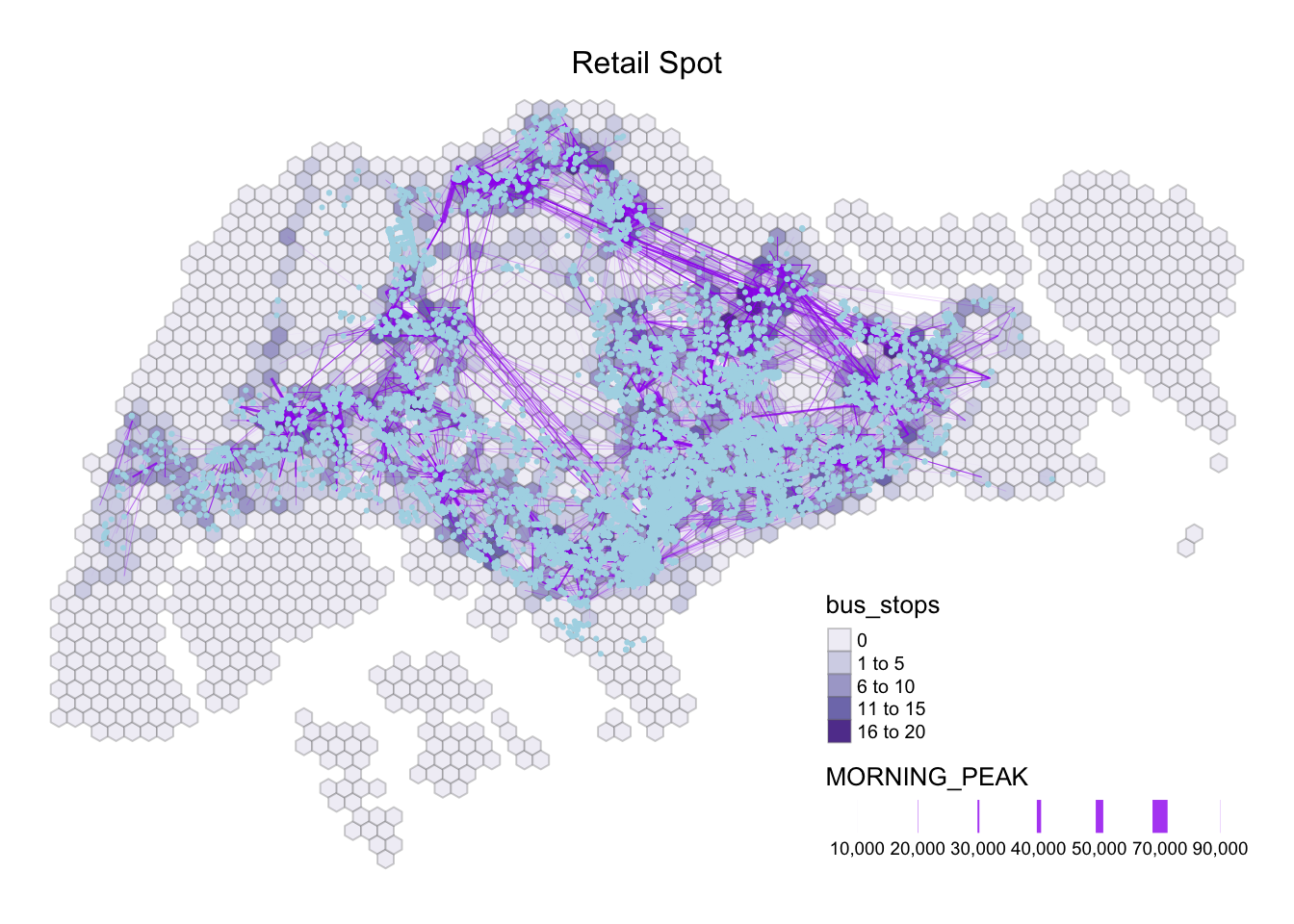
Show the code
#import school.csv into R environment
schools <- read_csv("data/aspatial/schools.csv") %>%
  rename(latitude = 'results.LATITUDE', longitude ='results.LONGITUDE') %>%
  select(postal_code, school_name, latitude, longitude)

#convert an aspatial data into sf tibble data frame
schools_sf <- st_as_sf(schools,
                       coords = c("longitude", "latitude"),
                       crs=4326) %>%
  st_transform(crs = 3414)

#plotting point symbol map with analytical hexagon grid
tmap_options(check.and.fix = TRUE)
tm_shape(hex_grid) +
  tm_fill(col = "bus_stops",palette = "Purples") +
tm_borders(alpha = 0.3) +
    flowLine %>%
    filter(MORNING_PEAK >= 1000) %>%
tm_shape() +
  tm_lines(lwd = "MORNING_PEAK",
           col = "purple",
           style = "quantile",
           scale = c(0.1, 1, 3, 5, 7, 10),
           n = 6,
           alpha = 0.8) +
    tm_layout(main.title = "Commuting flow of \n passengers with >1,000 trips",
            main.title.position = "center",
            main.title.size = 1,
            legend.height = 0.35,
            legend.width = 0.35,
            legend.outside = FALSE,
            legend.position = c("right", "bottom"),
            frame = FALSE) +
tm_shape(schools_sf) +
  tm_dots(col = "lightblue") +
  tm_layout(main.title = "School Spot",
            main.title.position = "center",
            main.title.size = 1,
            legend.height = 0.35,
            legend.width = 0.35,
            legend.outside = FALSE,
            legend.position = c("right", "bottom"),
frame = FALSE) 
As we are focusing on the Weekday Morning Peak Period from 0600 to 0900, based on my own understanding, I would personally eliminate the Entertainment variables, and Leisure & Recreation as I believe that the operating hours then to begin near noon. However, if we look at the maps above, we could see that the Entertainment spot is clustered around the central region with a handful around Singapore. Thus, we will exclude Entertainment for further analysis.
Looking into the Leisure & Recreation tab, we noticed that there are more spots in this field than Entertainment. By looking at the data set we noticed that there are multiple gyms and recreation centres. However, both companies does not operate around the same time, which would affect the accuracy of the data. Upon a closer look on the data, we observed that there are handful of spot that falls besides the grid that contains a bus stop, making it seems inaccessible to commuters. Therefore, we will exclude Leisure and Recreation for further analysis.
While looking at the other variables, the Food & Beverage (F&B) spot and School spot caught my eyes. At first glance, I assumed the F&B includes stalls in Hawker Centres, or Coffee Shop as I was expecting a wide amount of network, knowing how Singaporean loves food and would queue for food. Afer a close examination at the data, it is based on fine dining, bar , and pub. Thus, we could safely assume that the operating hours begins from 11.00am. As such, we will exclude Food & Beverage from further analysis.
Moreover, it is interesting to note that the School spot intersects with multiple commuting flows with darker bus stop density and thick line width. Moving forward, we will focus on Business, Financial Services, HDB, Retail, and school as our propulsive and attractiveness variables.
3.2 Compute point-in-polygon count
After confirming the five variables, we will count the number of spot located inside the grid_id by performing a point-in-polygon count. We will used the length() of Base package and st_intersects() of sf package. Thereafter, we will compute and display the summary statistics of computed variables using summary().
Count number of Businesses in Hexagon Grid
hex_grid$`BUSINESS_COUNT`<- lengths(st_intersects(hex_grid, business_sf))Summary Statistics
summary(hex_grid$BUSINESS_COUNT) Min. 1st Qu. Median Mean 3rd Qu. Max.
0.000 0.000 0.000 3.368 1.000 126.000 Count number of Financial Services in Hexagon Grid
hex_grid$`finserv_COUNT`<- lengths(st_intersects(hex_grid, finserv_sf))Summary Statistics
summary(hex_grid$finserv_COUNT) Min. 1st Qu. Median Mean 3rd Qu. Max.
0.000 0.000 0.000 1.707 0.000 176.000 Count number of HDB in Hexagon Grid
Show the code
hdb_sf_units <- st_intersection(hdb_sf, hex_grid) %>%
  st_drop_geometry() %>%
  group_by(grid_id) %>%
  summarise(
    HDB_SUM = sum(total_dwelling_units)
  ) %>%
  ungroup()

hex_grid <- left_join(hex_grid, hdb_sf_units, by = "grid_id")
hex_grid$HDB_SUM <- replace_na(hex_grid$HDB_SUM, 0)
Summary Statistics
summary(hex_grid$HDB_SUM) Min. 1st Qu. Median Mean 3rd Qu. Max.
0.0 0.0 0.0 560.8 0.0 8324.0 Count number of Retails in Hexagon Grid
hex_grid$`retail_COUNT`<- lengths(st_intersects(hex_grid, retail_sf))Summary Statistics
summary(hex_grid$retail_COUNT) Min. 1st Qu. Median Mean 3rd Qu. Max.
0.00 0.00 0.00 19.35 6.00 1427.00 Count number of School in Hexagon Grid
hex_grid$`school_COUNT`<- lengths(st_intersects(hex_grid, schools_sf))Summary Statistics
summary(hex_grid$school_COUNT) Min. 1st Qu. Median Mean 3rd Qu. Max.
0.0000 0.0000 0.0000 0.1799 0.0000 5.0000 From the above, we noticed that there are excessive 0 values in the field of each variables. Notably, we would still transform this field with log(). Thus, additional step is required to ensure that the 0 will be replaced with a value that is between 0 and 1.
4. Distance Matrix
Before we continue with the previous section, we will compute a distance matrix. It is a table that shows the distance between pairs of locations. In our context, we want to see the distance between one hexagonal grid to another.
4.1 Converting from sf data.table to SpatialPolygons Data Frame
To begin, we will use sp::as.Spatial() to convert hex_grid from sf tabble data frame to SpatialPolygonsDataFrame of sp object.
hex_grid_sp <- as(hex_grid, "Spatial")
hex_grid_sp
class : SpatialPolygonsDataFrame
features : 1945
extent : 2292.538, 57042.54, 15315.71, 50606.24 (xmin, xmax, ymin, ymax)
crs : +proj=tmerc +lat_0=1.36666666666667 +lon_0=103.833333333333 +k=1 +x_0=28001.642 +y_0=38744.572 +ellps=WGS84 +towgs84=0,0,0,0,0,0,0 +units=m +no_defs
variables : 7
names : grid_id, bus_stops, BUSINESS_COUNT, finserv_COUNT, HDB_SUM, retail_COUNT, school_COUNT
min values : 1, 0, 0, 0, 0, 0, 0
max values : 999, 20, 126, 176, 8324, 1427, 5 4.2 Computing the distance matrix
Next, we compute the Euclidean distance between the centroids of the hexagonal grid with the use of spDists() of sp package. head() is also used to examine a 10x10 matrix.
Show the code
dist <- spDists(hex_grid_sp,
                longlat = FALSE)
head(dist, n=c(10, 10))
[,1] [,2] [,3] [,4] [,5] [,6] [,7] [,8]
[1,] 0.000 1299.038 2598.076 3897.114 5196.152 750.000 1984.313 3269.174
[2,] 1299.038 0.000 1299.038 2598.076 3897.114 750.000 750.000 1984.313
[3,] 2598.076 1299.038 0.000 1299.038 2598.076 1984.313 750.000 750.000
[4,] 3897.114 2598.076 1299.038 0.000 1299.038 3269.174 1984.313 750.000
[5,] 5196.152 3897.114 2598.076 1299.038 0.000 4562.072 3269.174 1984.313
[6,] 750.000 750.000 1984.313 3269.174 4562.072 0.000 1299.038 2598.076
[7,] 1984.313 750.000 750.000 1984.313 3269.174 1299.038 0.000 1299.038
[8,] 3269.174 1984.313 750.000 750.000 1984.313 2598.076 1299.038 0.000
[9,] 4562.072 3269.174 1984.313 750.000 750.000 3897.114 2598.076 1299.038
[10,] 5857.687 4562.072 3269.174 1984.313 750.000 5196.152 3897.114 2598.076
[,9] [,10]
[1,] 4562.072 5857.687
[2,] 3269.174 4562.072
[3,] 1984.313 3269.174
[4,] 750.000 1984.313
[5,] 750.000 750.000
[6,] 3897.114 5196.152
[7,] 2598.076 3897.114
[8,] 1299.038 2598.076
[9,] 0.000 1299.038
[10,] 1299.038 0.000From the matrix, we noted that the headers for the columns and row are not labelled . Therefore, we will add a label into the distance matrix.
4.2.1 Label of Column and Row headers
To tidy, we will create a list sorted according to the distance matrix by grid_id.
id_names <- hex_grid$grid_idNext, we will attach grid_id to row and column for distance matrix matching.
colnames(dist) <- paste0(id_names)
rownames(dist) <- paste0(id_names)
4.2.2 Pivoting distance value by Grid_ID
Then, we will pivot the distance matrix into a long table by using the row and column of grid_id.
distPair <- melt(dist) %>%
  rename(dist = value)
head(distPair, 10)
Var1 Var2 dist
1 1 1 0.000
2 2 1 1299.038
3 3 1 2598.076
4 4 1 3897.114
5 5 1 5196.152
6 6 1 750.000
7 7 1 1984.313
8 8 1 3269.174
9 9 1 4562.072
10 10 1 5857.687From the data frame above, we noticed that the intra-zonal distance within the zone is zero. As such, we will append a constant value to replace the intra-zonal distance of 0 by performing the following:
- Find out the minimum value of the distance by using
summary() - Input a constant distance value
- Rename original and destination fields
Show the code
# find minimum distance value
distPair %>%
  filter(dist > 0) %>%
  summary()
Var1 Var2 dist
Min. : 1 Min. : 1 Min. : 750
1st Qu.: 487 1st Qu.: 487 1st Qu.:10894
Median : 973 Median : 973 Median :17477
Mean : 973 Mean : 973 Mean :18932
3rd Qu.:1459 3rd Qu.:1459 3rd Qu.:25401
Max. :1945 Max. :1945 Max. :57862 Show the code
distPair$dist <- ifelse(distPair$dist == 0,
                        200, distPair$dist)

# to check the distPair data frame
distPair %>%
  summary()
Var1 Var2 dist
Min. : 1 Min. : 1 Min. : 200
1st Qu.: 487 1st Qu.: 487 1st Qu.:10894
Median : 973 Median : 973 Median :17477
Mean : 973 Mean : 973 Mean :18923
3rd Qu.:1459 3rd Qu.:1459 3rd Qu.:25401
Max. :1945 Max. :1945 Max. :57862 #to rename the fields
distPair <- distPair %>%
rename(orig = Var1,
dest = Var2)
#save output to rds format.
write_rds(distPair, "data/rds/distPair.rds") We determined that the the minimum distance is 750m. Although we could put any values that are smaller than 750m to represent the intra-zonal distance, we input an arbitrary value of 200m that is smaller than the radius of the hexagon. We will save a copy of distPair output to RDS and re-load it into the R environment.
distPair <- read_rds("data/rds/distPair.rds")4.3 Prepare flow data
To get the flow data, we will compute the flow movement between and within the hexagonal grid by using the code chunk below. Output will be saved as flow_data. In addition, we will use head() to display the top 10 data frame.
Show the code
flow_data <- od_data1 %>%
  group_by(ORIGIN_ID, DESTIN_ID) %>%
  summarize(TRIPS = sum(MORNING_PEAK))


head(flow_data,10)
# A tibble: 10 × 3
# Groups: ORIGIN_ID [3]
ORIGIN_ID DESTIN_ID TRIPS
<fct> <fct> <dbl>
1 21 49 1
2 21 60 2
3 21 69 2
4 21 82 1
5 21 86 56
6 29 60 13
7 29 86 37
8 40 72 1
9 40 87 32
10 40 100 94.3.1 Separate Intra-flow
We will use ifelse() function to add three new fields in the dataframe with the condition that if Origin ID match Destination ID , zero will be forced.
Show the code
flow_data$FlowNoIntra <- ifelse(
  flow_data$ORIGIN_ID == flow_data$DESTIN_ID,
  0, flow_data$TRIPS)
flow_data$offset <- ifelse(
  flow_data$ORIGIN_ID == flow_data$DESTIN_ID,
  0.000001, 1)

glimpse(flow_data)
Rows: 65,076
Columns: 5
Groups: ORIGIN_ID [820]
$ ORIGIN_ID <fct> 21, 21, 21, 21, 21, 29, 29, 40, 40, 40, 40, 41, 41, 41, 41…
$ DESTIN_ID <fct> 49, 60, 69, 82, 86, 60, 86, 72, 87, 100, 253, 40, 49, 50, …
$ TRIPS <dbl> 1, 2, 2, 1, 56, 13, 37, 1, 32, 9, 2, 21, 3, 5, 4, 1, 7, 36…
$ FlowNoIntra <dbl> 1, 2, 2, 1, 56, 13, 37, 1, 32, 9, 2, 21, 3, 5, 4, 1, 7, 36…
$ offset <dbl> 1, 1, 1, 1, 1, 1, 1, 1, 1, 1, 1, 1, 1, 1, 1, 1, 1, 1, 1, 1…4.3.2 Combine flow_data and distPair
Before we join the data, we have to ensure that the data type is identical. As seen above, the flow_data for the grids are in <fct> format. Therefore, we will look at distPair.
glimpse(distPair)Rows: 3,783,025
Columns: 3
$ orig <int> 1, 2, 3, 4, 5, 6, 7, 8, 9, 10, 11, 12, 13, 14, 15, 16, 17, 18, 19…
$ dest <int> 1, 1, 1, 1, 1, 1, 1, 1, 1, 1, 1, 1, 1, 1, 1, 1, 1, 1, 1, 1, 1, 1,…
$ dist <dbl> 200.000, 1299.038, 2598.076, 3897.114, 5196.152, 750.000, 1984.31…From the results above, we note that the orig and dest are in <int> format. Similar, to section 2.3, we need to convert the data type from <int> to <fct>. After converting, we will run glimpse() again to check .
Show the code
#convert distPair from int to fct
distPair$orig <- as.factor(distPair$orig)
distPair$dest <- as.factor(distPair$dest)

glimpse(distPair)
Rows: 3,783,025
Columns: 3
$ orig <fct> 1, 2, 3, 4, 5, 6, 7, 8, 9, 10, 11, 12, 13, 14, 15, 16, 17, 18, 19…
$ dest <fct> 1, 1, 1, 1, 1, 1, 1, 1, 1, 1, 1, 1, 1, 1, 1, 1, 1, 1, 1, 1, 1, 1,…
$ dist <dbl> 200.000, 1299.038, 2598.076, 3897.114, 5196.152, 750.000, 1984.31…Now, we are ready to perform a dplyr::left_join() to flow_data dataframe and distPair dataframe. The output will be saved as flow_data1.
flow_data1 <- flow_data %>%
  left_join (distPair,
             by = c("ORIGIN_ID" = "orig",
                    "DESTIN_ID" = "dest"))
4.4 Preparing Origin and Destination Attributes
Next, we will add the origin and destination attributes by joinining it to the hex_grid data. We will process in two steps:
Add Origin attrbitues through flow_data using hex_grid by performing
left_join()Using the previous result, perform another
left_join()to add destination attributes.
In addition, we tidy the data by renaming columns to include a prefix. Origin attributes will be re-labeled as ORIGIN_XX, while destination attributes will be re-labeled as DESTIN_XX. As we do not need the bus_stop count and geometry, we will drop the columns.
Show the code
#left join based on origin attributes
flow_data2 <- flow_data1 %>%
  left_join(hex_grid,
            by = c(ORIGIN_ID = "grid_id")) %>%
    rename(ORIGIN_BUSINESS = BUSINESS_COUNT,
         ORIGIN_FINSER = finserv_COUNT,
         ORIGIN_HDB = HDB_SUM,
         ORIGIN_RETAIL = retail_COUNT,
         ORIGIN_SCHOOLS =school_COUNT
         ) %>%
  select(-c(bus_stops))

#left join based on destination attributes
flow_data2 <- flow_data2 %>%
  left_join(hex_grid,
            by = c(DESTIN_ID = "grid_id")) %>%
    rename(DESTIN_BUSINESS = BUSINESS_COUNT,
         DESTIN_FINSER = finserv_COUNT,
         DESTIN_HDB = HDB_SUM,
         DESTIN_RETAIL = retail_COUNT,
         DESTIN_SCHOOLS =school_COUNT
         ) %>%
  select(-c(bus_stops)) %>%
  select(-c(10,16))
5. Calibrating Spatial Interaction Models
Spatial interaction describe quantitatively the flow of people, material, or information between locations in geographical space.In this section, we will be looking at gravity models using the glm() function in R, namely:
Unconstrained Spatial Interaction Model
Origin Constrained Spatial Interaction Model
Destination Constrained Spatial Interaction Model
Doubly Constrained Spatial Interaction Model
5.1 Visualizing dependent variable
Before we run our models, we will do a quick visualization to visualize the distribution, and the relation between the dependent variable and one of the key independent variable in Spatial Interaction Model, namely distance.
Show the code
ggplot(data = flow_data2,
       aes(x = TRIPS)) +
  geom_histogram() +
  labs(title ="Distribution of Dependent Variable") +
  theme_minimal()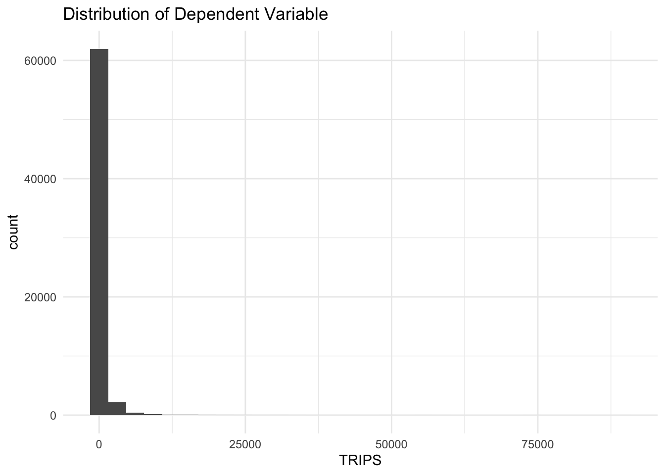
From the graph above, we noticed that the distribution is highly skewed and does not resembled a normal distribution. We will move on to visualize the relation.
Show the code
ggplot(data = flow_data2,
       aes(x = dist,
           y = TRIPS)) +
  geom_point() +
  geom_smooth(method = lm) +
  labs(title ="Relation between Dependent and Independent Variable") +
  theme_minimal()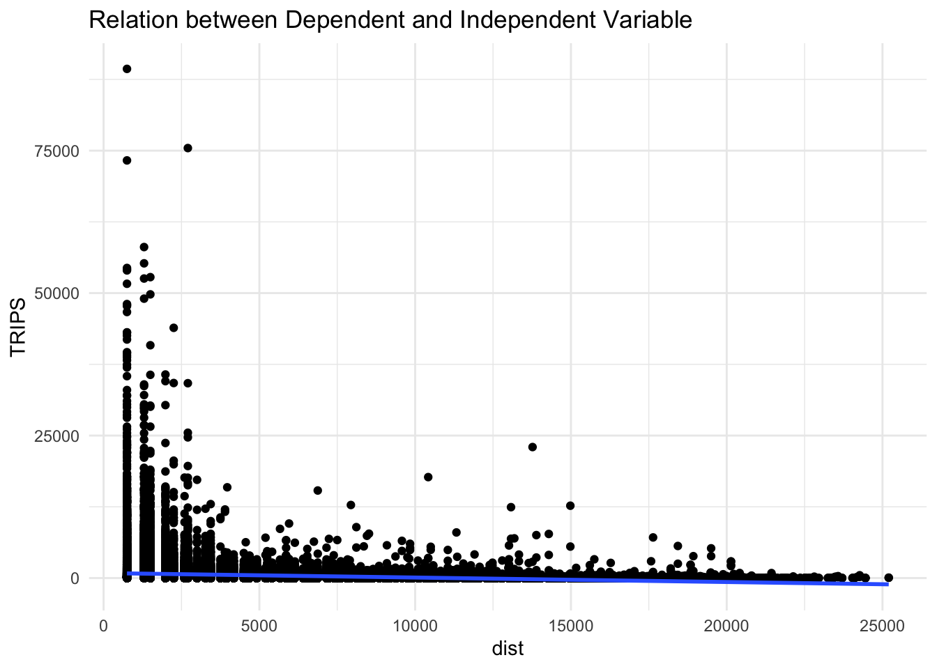
Based on the visualization above, it is difficult to determine if it resemble linear relationship. Therefore, we will use the log transformed version of both the dependent and independent variables, to see if they have a linear relationship.
Show the code
ggplot(data = flow_data2,
       aes(x = log(dist),
           y = log(TRIPS))) +
  geom_point() +
  geom_smooth(method = lm) +
  labs(title ="Relation between Dependent and Independent Variable (log)") +
  theme_minimal()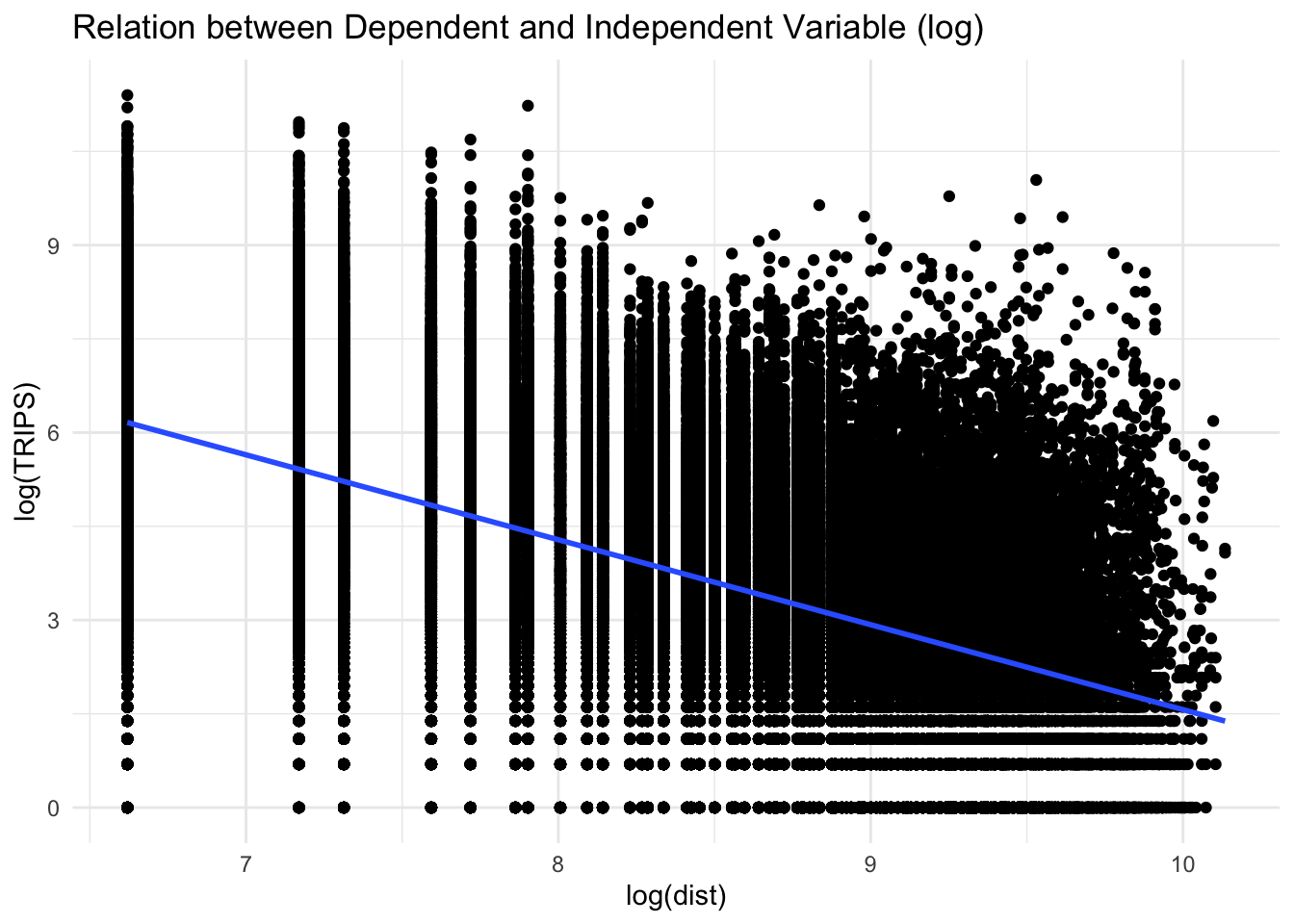
From the graph above, we are able to visualize a better linear relationship in comparison to the previous scatterplot. Also ,as observe earlier , we can confirmed that as the number of trips decreases, as the distance increases.
5.2 Checking for variables with zero values
Since Poisson Regression is based of log and log 0 is undefined, it is important for us to ensure to ensure that our exploratory variables does not contain any 0 values We will used the summary() of Base R to compute the summary statistics of all variables in the flow_data2 data frame.
summary(flow_data2) ORIGIN_ID DESTIN_ID TRIPS FlowNoIntra
1542 : 285 1234 : 364 Min. : 1.0 Min. : 1.0
1105 : 284 1210 : 355 1st Qu.: 7.0 1st Qu.: 7.0
1234 : 283 1233 : 342 Median : 37.0 Median : 37.0
1255 : 282 1212 : 317 Mean : 378.9 Mean : 378.9
1215 : 281 1542 : 299 3rd Qu.: 178.0 3rd Qu.: 178.0
1218 : 280 1105 : 298 Max. :89347.0 Max. :89347.0
(Other):63381 (Other):63101
offset dist ORIGIN_BUSINESS ORIGIN_FINSER ORIGIN_HDB
Min. :1 Min. : 750 Min. : 0.000 Min. : 0.000 Min. : 0
1st Qu.:1 1st Qu.: 3000 1st Qu.: 0.000 1st Qu.: 0.000 1st Qu.: 0
Median :1 Median : 5408 Median : 1.000 Median : 3.000 Median :1052
Mean :1 Mean : 6280 Mean : 6.571 Mean : 8.105 Mean :1848
3rd Qu.:1 3rd Qu.: 8842 3rd Qu.: 6.000 3rd Qu.: 8.000 3rd Qu.:3371
Max. :1 Max. :25200 Max. :126.000 Max. :176.000 Max. :8324
ORIGIN_RETAIL ORIGIN_SCHOOLS DESTIN_BUSINESS DESTIN_FINSER
Min. : 0.00 Min. :0.0000 Min. : 0.000 Min. : 0.000
1st Qu.: 7.00 1st Qu.:0.0000 1st Qu.: 0.000 1st Qu.: 0.000
Median : 29.00 Median :0.0000 Median : 1.000 Median : 3.000
Mean : 90.61 Mean :0.5865 Mean : 7.353 Mean : 8.997
3rd Qu.: 91.00 3rd Qu.:1.0000 3rd Qu.: 7.000 3rd Qu.: 9.000
Max. :1427.00 Max. :5.0000 Max. :126.000 Max. :176.000
DESTIN_HDB DESTIN_RETAIL DESTIN_SCHOOLS
Min. : 0 Min. : 0.00 Min. :0.0000
1st Qu.: 0 1st Qu.: 7.00 1st Qu.:0.0000
Median : 839 Median : 29.00 Median :0.0000
Mean :1741 Mean : 97.05 Mean :0.5577
3rd Qu.:3239 3rd Qu.: 97.00 3rd Qu.:1.0000
Max. :8324 Max. :1427.00 Max. :5.0000
From the summary statistics, we confirmed that we have removed intra-flow as the min of FlowNoIntra is 1. However, all our variables - ORIGIN_BUSINESS, ORIGIN_FINSER, ORIGIN_HDB, ORIGIN_RETAIL, ORIGIN_SCHOOLS, DESTIN_BUSINESS, DESTIN_FINSER, DESTIN_HDB, DESTIN_RETAIL, DESTIN_SCHOOLS contains 0 values.
As such, we will use the code chunk below to replace it with 0.99.
Show the code
#ORIGIN_BUSINESS
flow_data2$ORIGIN_BUSINESS <- ifelse(
  flow_data2$ORIGIN_BUSINESS == 0,
  0.99, flow_data2$ORIGIN_BUSINESS)

#ORIGIN_FINSER
flow_data2$ORIGIN_FINSER  <- ifelse(
  flow_data2$ORIGIN_FINSER == 0,
  0.99, flow_data2$ORIGIN_FINSER)

#ORIGIN_HDB
flow_data2$ORIGIN_HDB  <- ifelse(
  flow_data2$ORIGIN_HDB == 0,
  0.99, flow_data2$ORIGIN_HDB)

#ORIGIN_RETAIL
flow_data2$ORIGIN_RETAIL  <- ifelse(
  flow_data2$ORIGIN_RETAIL == 0,
  0.99, flow_data2$ORIGIN_RETAIL)

#ORIGIN_SCHOOLS
flow_data2$ORIGIN_SCHOOLS  <- ifelse(
  flow_data2$ORIGIN_SCHOOLS == 0,
  0.99, flow_data2$ORIGIN_SCHOOLS)

#DESTIN_BUSINESS
flow_data2$DESTIN_BUSINESS <- ifelse(
  flow_data2$DESTIN_BUSINESS == 0,
  0.99, flow_data2$DESTIN_BUSINESS)

#DESTIN_FINSER
flow_data2$DESTIN_FINSER  <- ifelse(
  flow_data2$DESTIN_FINSER == 0,
  0.99, flow_data2$DESTIN_FINSER)

#DESTIN_HDB
flow_data2$DESTIN_HDB  <- ifelse(
  flow_data2$DESTIN_HDB == 0,
  0.99, flow_data2$DESTIN_HDB)

#DESTIN_RETAIL
flow_data2$DESTIN_RETAIL  <- ifelse(
  flow_data2$DESTIN_RETAIL == 0,
  0.99, flow_data2$DESTIN_RETAIL)

#DESTIN_SCHOOLS
flow_data2$DESTIN_SCHOOLS  <- ifelse(
  flow_data2$DESTIN_SCHOOLS == 0,
  0.99, flow_data2$DESTIN_SCHOOLS)
To confirm , we re-run the summary() before saving the output in RDS format and re-load it into R.
summary(flow_data2) ORIGIN_ID DESTIN_ID TRIPS FlowNoIntra
1542 : 285 1234 : 364 Min. : 1.0 Min. : 1.0
1105 : 284 1210 : 355 1st Qu.: 7.0 1st Qu.: 7.0
1234 : 283 1233 : 342 Median : 37.0 Median : 37.0
1255 : 282 1212 : 317 Mean : 378.9 Mean : 378.9
1215 : 281 1542 : 299 3rd Qu.: 178.0 3rd Qu.: 178.0
1218 : 280 1105 : 298 Max. :89347.0 Max. :89347.0
(Other):63381 (Other):63101
offset dist ORIGIN_BUSINESS ORIGIN_FINSER
Min. :1 Min. : 750 Min. : 0.990 Min. : 0.990
1st Qu.:1 1st Qu.: 3000 1st Qu.: 0.990 1st Qu.: 0.990
Median :1 Median : 5408 Median : 1.000 Median : 3.000
Mean :1 Mean : 6280 Mean : 6.986 Mean : 8.375
3rd Qu.:1 3rd Qu.: 8842 3rd Qu.: 6.000 3rd Qu.: 8.000
Max. :1 Max. :25200 Max. :126.000 Max. :176.000
ORIGIN_HDB ORIGIN_RETAIL ORIGIN_SCHOOLS DESTIN_BUSINESS
Min. : 0.99 Min. : 0.99 Min. :0.990 Min. : 0.990
1st Qu.: 0.99 1st Qu.: 7.00 1st Qu.:0.990 1st Qu.: 0.990
Median :1052.00 Median : 29.00 Median :0.990 Median : 1.000
Mean :1848.02 Mean : 90.67 Mean :1.183 Mean : 7.747
3rd Qu.:3371.00 3rd Qu.: 91.00 3rd Qu.:1.000 3rd Qu.: 7.000
Max. :8324.00 Max. :1427.00 Max. :5.000 Max. :126.000
DESTIN_FINSER DESTIN_HDB DESTIN_RETAIL DESTIN_SCHOOLS
Min. : 0.990 Min. : 0.99 Min. : 0.99 Min. :0.990
1st Qu.: 0.990 1st Qu.: 0.99 1st Qu.: 7.00 1st Qu.:0.990
Median : 3.000 Median : 839.00 Median : 29.00 Median :0.990
Mean : 9.266 Mean :1740.90 Mean : 97.12 Mean :1.173
3rd Qu.: 9.000 3rd Qu.:3239.00 3rd Qu.: 97.00 3rd Qu.:1.000
Max. :176.000 Max. :8324.00 Max. :1427.00 Max. :5.000
5.3 Unconstrained Spatial Interaction Model
The first model that we will looking at will be the Unconstrained model. There are no external restrictions on the flow value. Thus, any origin can send flows to any destination based solely on the attraction potential of the destination and the distance. We will save the output - uncSIM into a RDS format.
Show the code
uncSIM <- glm(formula = TRIPS ~
                log(ORIGIN_BUSINESS) +
                log(DESTIN_BUSINESS) +
                log(ORIGIN_FINSER) +
                log(DESTIN_FINSER) +
                log(ORIGIN_HDB) +
                log(DESTIN_HDB) +
                log(ORIGIN_RETAIL) +
                log(DESTIN_RETAIL) +
                log(ORIGIN_SCHOOLS) +
                log(DESTIN_SCHOOLS) +
                log(dist),
              family = poisson(link = "log"),
              data = flow_data2,
              na.action = na.exclude)
#save RDS
write_rds(uncSIM, "data/rds/uncSIM.rds")
As we are not executing the code chunk above, we will load uncSIM into the R environment.
Also, we will run uncSIM to view the result.
uncSIM
Call:  glm(formula = TRIPS ~ log(ORIGIN_BUSINESS) + log(DESTIN_BUSINESS) +
    log(ORIGIN_FINSER) + log(DESTIN_FINSER) + log(ORIGIN_HDB) +
    log(DESTIN_HDB) + log(ORIGIN_RETAIL) + log(DESTIN_RETAIL) +
    log(ORIGIN_SCHOOLS) + log(DESTIN_SCHOOLS) + log(dist), family = poisson(link = "log"),
    data = flow_data2, na.action = na.exclude)

Coefficients:
         (Intercept)  log(ORIGIN_BUSINESS)  log(DESTIN_BUSINESS)
            16.04170              -0.13531               0.04363
  log(ORIGIN_FINSER)    log(DESTIN_FINSER)       log(ORIGIN_HDB)
             0.16080               0.31340               0.15163
     log(DESTIN_HDB)    log(ORIGIN_RETAIL)    log(DESTIN_RETAIL)
             0.01262              -0.03330               0.01250
 log(ORIGIN_SCHOOLS)   log(DESTIN_SCHOOLS)             log(dist)
             0.27070               0.41777              -1.46077

Degrees of Freedom: 65075 Total (i.e. Null);  65064 Residual
Null Deviance:      98390000
Residual Deviance: 50260000     AIC: 50610000
Goodness of fit
With the aid of R-squared statistics , we will write a function called CalcRSquared to compute the proportion of variance in the dependent variables. The R2 indicates the degree to which the model explains the observed variation in the dependent variable, relative to the mean. The R2 always lies between 0 and 1, where a higher R2 indicates a better model fit.
#create function to calculate r-squared value
CalcRSquared <- function(observed,estimated){
  r <- cor(observed,estimated)
  R2 <- r^2
  R2
}
After we create the function, we can examine how the constraints hold.
CalcRSquared(uncSIM$data$TRIPS, uncSIM$fitted.values)[1] 0.2214091With reference to the R-squared above, we can conclude that the model accounts for about 22% of the variation of flows in the system. Since the p-value is less than the alpha of 0.05, we will reject the null hypothesis that the mean is a good estimator for the explanatory variables. However, it does not bring in more insights on which variables to look at since the value of R2 tells that the ten explanatory variables can account for 22% of the variation.
5.4 Origin (Production) constrained SIM
The second model that we are looking at will be the Origin Constrained model. The flow value are based on the destination attributes. We will save the output - orcSIM into a RDS format and re-load into the R environment.
Show the code
orcSIM <- glm(formula = TRIPS ~
                 ORIGIN_ID +
                 log(DESTIN_BUSINESS) +
                 log(DESTIN_FINSER) +
                 log(DESTIN_HDB) +
                 log(DESTIN_RETAIL) +
                 log(DESTIN_SCHOOLS) +
                 log(dist),
              family = poisson(link = "log"),
              data = flow_data2,
              na.action = na.exclude)
#save RDS
write_rds(orcSIM, "data/rds/orcSIM.rds")
As we are not executing the code chunk above, we will load orcSIM into the R environment.
orcSIM <- read_rds("data/rds/orcSIM.rds")Click on to view the summary statistics of orcSIM.
Goodness of fit
With the aid of R-squared statistics , we will compute the proportion of variance in the dependent variables.
CalcRSquared(orcSIM$data$TRIPS, orcSIM$fitted.values)[1] 0.3257997With reference to the R-squared above, we can conclude that the model accounts for about 33% of the variation of flows in the system. The value of R2 tells that the five DESTIN explanatory variables can account for 33% of the variation. In addition, the p-value is less than the alpha of 0.05, we will reject the null hypothesis that the mean is a good estimator for the five DESTIN variables.
Looking at the explanatory variables, we note that Retail contributed the most in commuting flow , followed by Business, Schools, and Financial Service. We also note that their relationship are not the same as HDB results in negative value.As such, we are to infer that housing location (HDB) is a propulsive factor.
5.5 Destination constrained SIM
The third model that we are looking at will be the Destination Constrained model. The flow value are based on the origin attributes. We will save the output - decSIM into a RDS format and re-load into the R environment.
Show the code
decSIM <- glm(formula = TRIPS ~
                DESTIN_ID +
                log(ORIGIN_BUSINESS) +
                log(ORIGIN_FINSER) +
                log(ORIGIN_HDB) +
                log(ORIGIN_RETAIL) +
                log(ORIGIN_SCHOOLS) +
                log(dist),
              family = poisson(link = "log"),
              data = flow_data2,
              na.action = na.exclude)
#save RDS
write_rds(decSIM, "data/rds/decSIM.rds")
As we are not executing the code chunk above, we will load decSIM into the R environment.
decSIM <- read_rds("data/rds/decSIM.rds")Click on to view the summary statistics of decSIM.
Goodness of fit
With the aid of R-squared statistics , we will compute the proportion of variance in the dependent variables.
CalcRSquared(decSIM$data$TRIPS, decSIM$fitted.values)[1] 0.3991156With reference to the R-squared above, we can conclude that the model accounts for about 40% of the variation of flows in the system. In addition, the p-value is less than the alpha of 0.05, we will reject the null hypothesis that the mean is a good estimator for the five ORIGIN variables.
Looking at the explanatory variables, we note that Retail contributed the most in commuting flow , followed by Schools, Financial Service, and HDB. We also note that their relationship are not the same as Business results in negative value. We could infer that most people commute to Retail spot followed by Schools.
5.6 Doubly constrained SIM
The last model that we are looking at will be the Doubly Constrained model. The flow value are not pre-determined. We will save the output - dbcSIM into a RDS format and re-load into the R environment.
Show the code
dbcSIM <- glm(formula = TRIPS ~
                ORIGIN_ID +
                DESTIN_ID +
                log(dist),
              family = poisson(link = "log"),
              data = flow_data2,
              na.action = na.exclude)
#save RDS
write_rds(dbcSIM, "data/rds/dbcSIM.rds")
As we are not executing the code chunk above, we will load orcSIM into the R environment.
dbcSIM <- read_rds("data/rds/dbcSIM.rds")Click on to view the summary statistics of dbcSIM.
Goodness of fit
With the aid of R-squared statistics , we will compute the proportion of variance in the dependent variables.
CalcRSquared(dbcSIM$data$TRIPS, dbcSIM$fitted.values)[1] 0.5737163With reference to the R-squared (R2) above, we can conclude that the model accounts for about 57% of the variation of flows in the system. In addition, the p-value is <0.05, we can reject the null hypothesis. We also note that there is a relatively improvement in the R2 value.
5.7 Model Comparison
After running all models, we will use another statistical measures to compare the performance. We will be using performance:compare_performance() to measure the Root Mean Squared Error (RMSE). Generally, when we look at RMSE, the performance is better when the number is smaller.
model_list <- list(unconstrained=uncSIM,
                   originConstrained=orcSIM,
                   destinationConstrained=decSIM,
                   doublyConstrained=dbcSIM)
Next, we will compute the RMSE of all the models in model_list file by using the code chunk below.
compare_performance(model_list,
                    metrics = "RMSE")
# Comparison of Model Performance Indices
Name | Model | RMSE
-----------------------------------------
unconstrained | glm | 1587.446
originConstrained | glm | 1476.694
destinationConstrained | glm | 1394.096
doublyConstrained | glm | 1175.151By looking at the results, we note that the R2 and RMSE are consistent as both shows doubly constrained SIM as the preferred model. It has the highest R2 results, and the lowest RMSE value of 1,175.151.
5.8 Visualize Fitting
After running the models and comparing the result, we will visualize the observed values and the fitted values.
First, we will extract the fitted values from each model.
#extract fitted values
df <- as.data.frame(uncSIM$fitted.values) %>%
  round(digits = 0)

#append fitted values
flow_data2 <- flow_data2 %>%
  cbind(df) %>%
  rename(uncTRIPS = "uncSIM$fitted.values")
#extract fitted values
df <- as.data.frame(orcSIM$fitted.values) %>%
round(digits = 0)
#append fitted values
flow_data2 <- flow_data2 %>%
cbind(df) %>%
rename(orcTRIPS = "orcSIM$fitted.values")#extract fitted values
df <- as.data.frame(decSIM$fitted.values) %>%
round(digits = 0)
#append fitted values
flow_data2 <- flow_data2 %>%
cbind(df) %>%
rename(decTRIPS = "decSIM$fitted.values")#extract fitted values
df <- as.data.frame(dbcSIM$fitted.values) %>%
round(digits = 0)
#append fitted values
flow_data2 <- flow_data2 %>%
cbind(df) %>%
rename(dbcTRIPS = "dbcSIM$fitted.values")5.8.1 Scatterplot
Then, we will use geom_point() of ggplot2 package to create our scatterplots.
Show the code
unc_p <- ggplot(data = flow_data2,
                aes(x = uncTRIPS,
                    y = TRIPS)) +
  geom_point() +
  geom_smooth(method = lm) +
  theme_minimal()

orc_p <- ggplot(data = flow_data2,
                aes(x = orcTRIPS,
                    y = TRIPS)) +
  geom_point() +
  geom_smooth(method = lm) +
    theme_minimal()

dec_p <- ggplot(data = flow_data2,
                aes(x = decTRIPS,
                    y = TRIPS)) +
  geom_point() +
  geom_smooth(method = lm) +
    theme_minimal()

dbc_p <- ggplot(data = flow_data2,
                aes(x = dbcTRIPS,
                    y = TRIPS)) +
  geom_point() +
  geom_smooth(method = lm) +
    theme_minimal()

#arrange graphs
plot <- ggarrange(unc_p, orc_p, dec_p, dbc_p,
          ncol = 2,
          nrow = 2)

#add title
annotate_figure(plot, top = text_grob("Scatterplots across SLM Models"))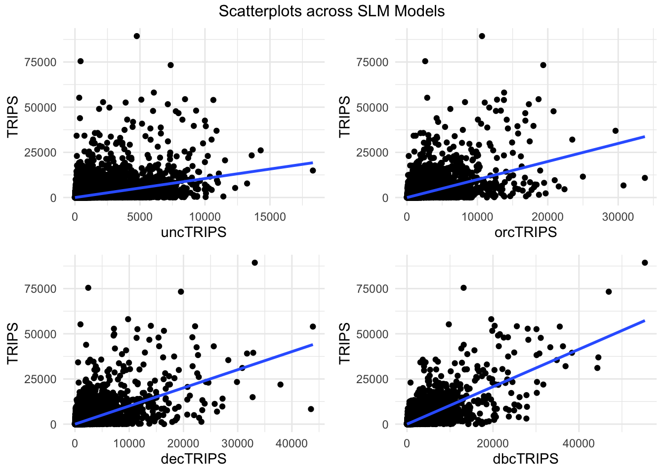
The plot above reveals that there are a few statistical outliers that have relatively frequent trips. The slope seems to be smoother for uncTRIPs, followed by orcTRIPs and gradually, become steeper. All of the models have positive correlation.
6. Conclusion and Future Work
In our exercise, we examine the urban mobility patterns of commuters on the time period of Weekday Morning 0600 -0900 by looking at the explanatory variables - Business, Financial Service, HDB, Retail, and School based on hexagonal grid. We used Spatial Interaction Models and found out that the Doubly Constrained SIM yields better results in R2 and RMSE.
To improve our study, after the initial stage of exploring the model, we could perform stepwise regression by adding and removing independent variables, in the predictive model, in order to find the subset of variables in the data set which results in the best performing model. However, it is important to note that adding variables might improve the score of R2, it might causes overfitting issues.
References:
Land Transport Authority. (2023). DataMall. Retrieved from https://datamall.lta.gov.sg/content/datamall/en.html
Wong, K. (2021, August). Tessellation SF: A Map Design Pattern. Retrieved from https://urbandatapalette.com/post/2021-08-tessellation-sf